Problem Setup

Suppose that we want to predict salary based on age, education, gender, job, etc, the common way to set up this problem is to represent the $n$ data points with $m$ features as a matrix:

$$ X = \begin{pmatrix} x_{1,1} & x_{1,2} & \cdots & x_{1,m} \\ x_{2,1} & x_{2,2} & \cdots & x_{2,m} \\ \vdots & \vdots & \ddots & \vdots \\ x_{n,1} & x_{n,2} & \cdots & x_{n,m} \end{pmatrix} $$

where $x_{i,1}, x_{i,2}, x_{i,3}, ...$ could be the age, education, job and other features for the $i$-person.

We could also represent the salaries for each person as a vector:

$$ y = \begin{pmatrix} y_1 \\ y_2 \\ \vdots \\ y_n \end{pmatrix} $$

Thus linear regression can be thought of finding another vector

$$ \beta = \begin{pmatrix} \beta_1 \\ \beta_2 \\ \vdots \\ \beta_m \end{pmatrix} $$

such that $$ X\beta \approx y $$

We shall define the approximation $\approx$ rigorously later.

Some Linear Algebra

Given that $X \in \mathbb{R}^{n,m}$, the set $\{Xu| u \in \mathbb{R}^m\}$ forms a linear subspace.

Example 1: Suppose that

$$ X= \begin{pmatrix} 1 \\ 2 \\ \end{pmatrix} $$

then the set $\{Xu| u \in \mathbb{R}\}$ is a straight line

Example 2: Suppose that

$$ X= \begin{pmatrix} 1 & 4\\ 2 & 5 \\ 3 & 6 \end{pmatrix} $$

then set $\{Xu| u \in \mathbb{R}^2\}$ is a plane

In general, the set $\{Xu| u \in \mathbb{R}^m\}$ is a hyperplane. So if $y$ is on the hyperplane, then by definition there is a $\beta \in \mathbb{R}^m$ that can satisfy the equation $X\beta=y$.

Now suppose $y$ is not on the hyperplane, next best thing we can do is to find a $\hat{y}$ on the hyperplabe that is closest to $y$, which is the orthogonal projection of $y$ onto the plane .

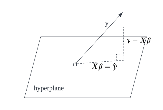
By the definition of orthogonality, we know that

$$ X^T(y-X\beta) = 0 \\ $$

and thus $$ \beta = (X^TX)^{-1}X^Ty $$

This is the analytical solution of our linear regression problem.

Coding Examples using Julia

Now let's try some concrete example to see if it actually works. Let's generate 100 random points using the real $\beta=0.2$ and some random noise, and figure out if we can recover the $\beta$ using only $X$ and $y$

X = randn(100)
β = 0.2
y = X*β + randn(100)/10
scatter(X, y)

Now we can calculate using the formula

(X'*X)^-1*X'*y

0.19280849762611454

0.19 is really close to 2 (the real $\beta$) ! The same formula hold for higher dimension. We can't visualize it, but we can perform the calculation as usual.

X = randn(100,5)
β = [0.1,0.2,0.3,0.4,0.5]
y = X*β + randn(100)/10

(X'*X)^-1*X'*y

5-element Vector{Float64}:
 0.08658415160224578
 0.19121983641861673
 0.31556448265297393
 0.4116056101763966
 0.49374419922975754

observe that $(0.08, 0.19, 0.32, 0.41, 0.49)$ is really close to $(0.1,0.2,0.3,0.4,0.5)$.